Pattern Recognition at Home

This article was originally published on April 22, 2020 on medium.com

Картинка

Peter Brueghel the Younger. “The village alchemist”

You have probably already met on Twitter or LinkedIn with a meme where COVID-19 is indicated as accountable for the digital transformation of a company.

Digitalization, as with COVID-19 mostly, may lie in transferring of staff and of processes online. However, while everyone is familiar with e-mail, browsers, or software like Zoom, many heard about machine learning, and neural networks by name only. So in this article, I suggest you get acquainted with applications of artificial intelligence, probably the most promising area of digitalization.

Nowadays, almost everyone can deal with some simple AI tasks. The recipe is rather simple: take some ready-made implementation of neural network architecture such as Mask R-CNN, add a little bit of code and run it on Google Colab.

For instance, with just a few lines of code, you can change in a photo of party balloons the color of the background to black and white …

Картинка

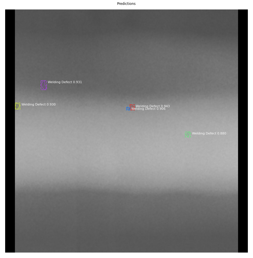
… or detect weld defects in an X-ray image

Картинка

Next, I will try to show you how to get the same results by yourself.

These step-by-step instructions will be of interest to those who would like to create some neural network applications with minimal effort.

In the first part, you’ll get instructed for using a trained model for replacing the color background of images of party balloons with black and white. The second part — is for training and testing of a model for weld defects detection in X-ray images.

Part 1. Processing Images of Party Balloons

Let’s get started with the simplest task — launching a trained and ready-to-use model.

First, create a new notebook on Google Colab.

Картинка

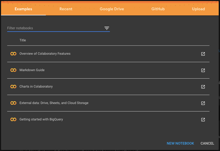
Collaboratory, or “Collab” for short, allows you to write and execute Python in your browser. In “Collab”, the environment for running Python code works out-of-the-box, you get a free graphics accelerator such as NVidia Tesla K80.

TensorFlow 1.x is required in the model used, therefore, in order to avoid code execution errors, we indicate the required version in the very first line.

A new code cell can be created by keys Ctrl + A (new cell above)/Ctrl + В (new cell below), or by clicking + Code under the main bar, or by Insert menu.

# run this cell once again in case of error "AttributeError: module 'tensorflow' has no attribute 'placeholder'" 
%tensorflow_version 1.x

Code is executed line by line by pressing the key Ctrl + Enter, whole code - by the keys Ctrl + F9

Next, specify the URL for an image of balloons. You can easily replace it with yours.

# to use custom image with balloons change the link below
balloon_URL = 'https://live.staticflickr.com/2677/4404039169_042fa233d1_b.jpg'

Clone the repository of the Mask R-CNN model.

# download Mask RCNN model 
!git clone [https://github.com/matterport/Mask_RCNN.git](https://github.com/matterport/Mask_RCNN.git)

Next, select the directory with our model instance cloned.

# choose MaskRCNN folder %cd /content/Mask_RCNN/

In the selected directory, download the model trained for balloon image recognition.

# download Mask RCNN Balloon model weigths 
!pip install wget 
import wget wget.download('https://github.com/matterport/Mask_RCNN/releases/download/v2.1/mask_rcnn_balloon.h5')

Selecting the directory where the balloon.py file with the code for our model is located

# choose directory with balloon.py file # run this cell once again in case of error "python3: can't open file 'balloon.py': [Errno 2] No such file or directory" 
%cd /content/Mask_RCNN/samples/balloon

Next, we actually run the command, which performs the Splash function from the ballon.py file, using the weights of the trained model from the mask_rcnn_balloon.h5 file, and processes the image at the link specified by us.

%%capture cap_out 
!python balloon.py splash \
--weights=/content/Mask_RCNN/mask_rcnn_balloon.h5 \ 
--image=$balloon_URL

And then, after that, we can compare the original and processed images using the code below.

# plot original and modified images 
%pylab inline 
from PIL import Image 
import matplotlib.pyplot as plt 
import matplotlib.image as mpimg 
import requests 
img_orig = Image.open(requests.get(balloon_URL, stream=True).raw) img_splash=mpimg.imread(cap_out.stdout.split()[-1]) 
fig = plt.figure(figsize=(20,10)) 
ax1 = fig.add_subplot(1,2,1) 
ax1.set_title('Original') 
ax1.imshow(img_orig) 
ax2 = fig.add_subplot(1,2,2) 
ax2.set_title('Modified') 
ax2.imshow(img_splash) 
plt.show()

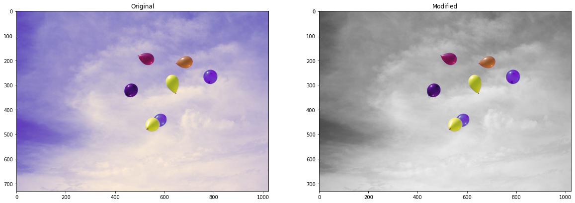
Output

Output

Part 2. Looking for Weld Defects in X-Rays Images

Here we use the defect detection system which is a fork of Matterport Mask RCNN used in the previous task.

Unlike the previous task, we will train a model. There are restrictions on using Google Colab. The time of Colab virtual machine sessions is limited to a maximum of 12 hours of use, after which all data is reset. The training takes a total of about 26 hours of machine time to carry on. Therefore, we will need to create checkpoints (configured by default), and Google Drive is well-suited for storing them.

Google Drive provides for free 15 GiB of disk space, the total amount of space occupied by control points after 160 epochs of training can be 38 GiB. Thus, as the disk becomes full, it is necessary to free up space by deleting previous checkpoints (except the last one) or increase the storage limit by subscribing to Google One (checkpoints may be used for data visualization in Tensorboard).

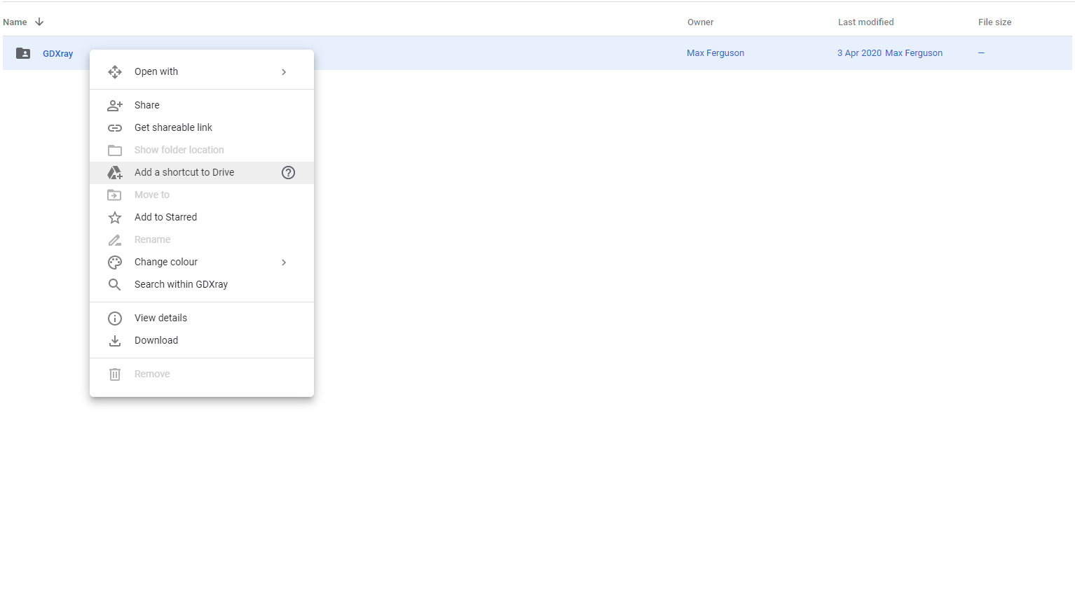
Google Drive

First, add a shortcut to the folder with the GDXray data set on your Drive disk. This will allow us not to download this dataset and not to occupy disk space.

Colab

As in the previous task, create a new notebook.

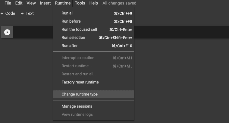
On Colab, a CPU is used as default runtime. To train a model, a GPU or a TPU accelerator should be chosen. Google claims TPU makes calculations faster compared to GPU, but it requires the model to be tuned for TPU.

Choosing runtime type (Runtime > Change runtime type).

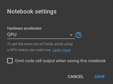
Select a GPU graphics accelerator in the drop-down list.

Connect to a virtual machine using the button Connect.

Choose the required version of TensorFlow.

#run this cell once again in case of error "AttributeError: module 'tensorflow' has no attribute 'placeholder'" 
%tensorflow_version 1.x

Here, we need to configure the environment by specifying libraries version.

Libraries version is taken from environment.yml file. This file is used to configure an environment in Anaconda.

!pip install scipy==1.1.0 
!pip install opencv-python==4.1.0.25 
!pip install tensorflow-gpu==1.5 
!pip install keras==2.1.3

To connect to Google Drive get an authorization code by a link that appears.

from google.colab import drive 
drive.mount('/content/gdrive', force_remount=True)

Select the mounted Google Drive disk.

%cd gdrive/My\ Drive

Clone (download to a Google Drive) the repository of the Metal defect detection project.

!git clone [https://github.com/maxkferg/metal-defect-detection.git](https://github.com/maxkferg/metal-defect-detection.git)

Select the directory into which the instance was cloned.

# choose MaskRCNN folder 
%cd /content/gdrive/My\ Drive/metal-defect-detection

Here transfer learning is used which means a model trained on one task is re-purposed on a second related task thus we load mask_rcnn_coco.h5 file with weights of a model pre-trained on the COCO dataset.

# download COCO model weigths 
!pip install wget 
import wget wget.download('https://github.com/matterport/Mask_RCNN/releases/download/v2.0/mask_rcnn_coco.h5')

Start training.

!python gdxray.py train \ 
--dataset=/content/gdrive/My\ Drive/GDXray/GDXray \ 
--series=All \ 
--model=mask_rcnn_coco.h5 \ 
--logs=logs/gdxray \ 
--download=True

As I have already pointed out, the learning process takes a quite long time, and restarting may be required if a runtime session is reset. In this case, run a cell with the following code.

# run this cell after runtime restarting 
%tensorflow_version 1.x 
!pip install scipy==1.1.0 
!pip install opencv-python==4.1.0.25 
!pip install tensorflow-gpu==1.5 
!pip install keras==2.1.3 from google.colab import drive drive.mount('/content/gdrive', force_remount=True) 
%cd /content/gdrive/My\ Drive/metal-defect-detection 
!python gdxray.py train \ 
--dataset=/content/gdrive/My\ Drive/GDXray/GDXray \ 
--series=All \ 
--model=last \ 
--logs=logs/gdxray \ 
--download=False

Training ends after 160 epochs. There is a notebook inspect_model.ipynb in the project directory to visualize how the model works. A link posted a slightly modified file. I have added some code to work with Google Drive and a code block to upload images via URL.

Defect Detecting Results

Original image

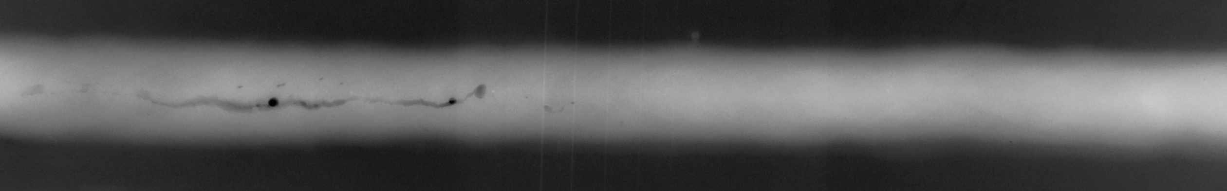
Original image

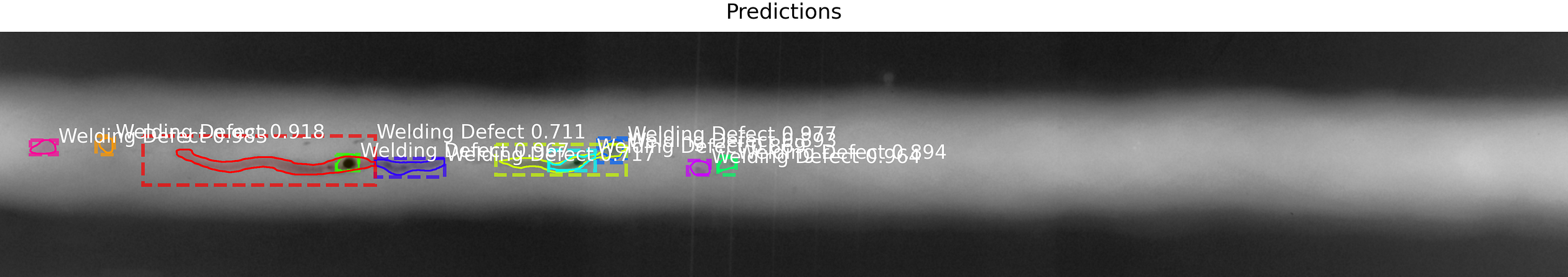
Processed image

Processed image

In Conclusion

The performance of GPUs is increasing every day, algorithms are improving, and access to technologies is simplified. All this expands the range of users and the scope of neural network applications.

By way of example, I presented the tasks of processing photographs and detecting defects in X-ray images — not very suitable for everyday life, admittedly. Although, actually, there are more practical things, such as snagging parking spaces or doorbell cameras with a built-in face recognition system. Try it, neural networks and powerful graphics accelerators are available to everyone nowadays.

Pattern Recognition at Home

Part 1. Processing Images of Party Balloons

Links

Part 2. Looking for Weld Defects in X-Rays Images

Google Drive

Colab

Defect Detecting Results

Links

In Conclusion